Overview
In my last post, I ended up using Windowing to enhance the Fourier analysis of my audio signal. I wanted to spend some more time playing with this, and since this is a learning exercise, not product development, I can choose to chase after shiny things!
Today I’d like to understand a bit more the effects of various windows.
Reference Signal
I’m going to create an ideal signal for this exercise – I’ll use the same 1kHz signal that my DAC was creating. As a starting point, I’m going to plot the FFT of this signal.
def reference_analysis():
    sample_rate_hz = 192 * 1000
    sample_time_s = 1.0/sample_rate_hz
    duration_s = 1
    n_samples = sample_rate_hz * duration_s
    amplitude_V = 6
    freq_hz = 1 * 1000
    t = np.linspace(0, duration_s - sample_time_s, num=n_samples)
    s = amplitude_V * np.sin(2 * np.pi * freq_hz * t)

    # Plot the ideal window signal
    s_fft = scipy.fftpack.rfft(s) * 2 / len(s)
    f_fft = scipy.fftpack.rfftfreq(len(s_fft), d=1 / sample_rate_hz)
    plt.plot(f_fft, 20*np.log10(np.abs(s_fft)), label='Ideal sample window')

    plt.xlabel('Frequency (Hz)')
    plt.ylabel('dBV')
    plt.xscale('log')
    plt.xlim([20, 20000])
    plt.grid(True, which='both')
    plt.title('Spectrum (dBV) vs Frequency (Hz) of 1kHz sine wave')

    plt.legend()
    plt.show()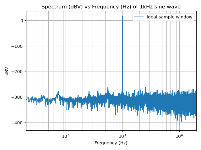
This effectively uses what is called a Rectangular Window – think of it as just multiplying each sample by 1. In this carefully controlled example, the signal to noise appears to be around -300dBV (or around 1e-15V). This is because I carefully chose the samples to use, and ensured that they are a continuous subset of the wave (i.e. the end of the loop lines up correctly with the beginning of the loop). If you were to copy-and-paste these samples, it would make a very smooth and clean sine wave. These 192000 samples contain 192 cycles of the 1kHz wave.
Real World
In the real world, we don’t have this luxury; the samples that we take aren’t likely to be continuous in this way. We can simulate this by grabbing a subset of the samples that do not nicely coincide: I chose to lop off some samples at the beginning and end of the wave and plot this modified sample window:
def reference_analysis():
    sample_rate_hz = 192 * 1000
    sample_time_s = 1.0/sample_rate_hz
    duration_s = 1
    n_samples = sample_rate_hz * duration_s
    amplitude_V = 6
    freq_hz = 1 * 1000
    t = np.linspace(0, duration_s - sample_time_s, num=n_samples)
    s = amplitude_V * np.sin(2 * np.pi * freq_hz * t)

    # Plot the ideal window signal
    s_fft = scipy.fftpack.rfft(s) * 2 / len(s)
    f_fft = scipy.fftpack.rfftfreq(len(s_fft), d=1 / sample_rate_hz)
    plt.plot(f_fft, 20*np.log10(np.abs(s_fft)), label='Ideal sample window')

    # Drop some samples at the beginning and end of the ideal samples
    first_sample = 101
    last_sample = len(s) - 67
    print('{} - {}'.format(first_sample, last_sample))
    windowed_samples = s[first_sample:last_sample]
    window_fft = scipy.fftpack.rfft(windowed_samples) * 2 / len(windowed_samples)
    f_window_fft = scipy.fftpack.rfftfreq(len(window_fft), d=1/sample_rate_hz)

    # Plot the FFT of the modified sample window
    plt.plot(f_window_fft, 20*np.log10(np.abs(window_fft)), color='r', label='Offset sample window')

    plt.xlabel('Frequency (Hz)')
    plt.ylabel('dBV')
    plt.xscale('log')
    plt.xlim([20, 20000])
    plt.grid(True, which='both')
    plt.title('Spectrum (dBV) vs Frequency (Hz) of 1kHz sine wave')

    plt.legend()
    plt.show()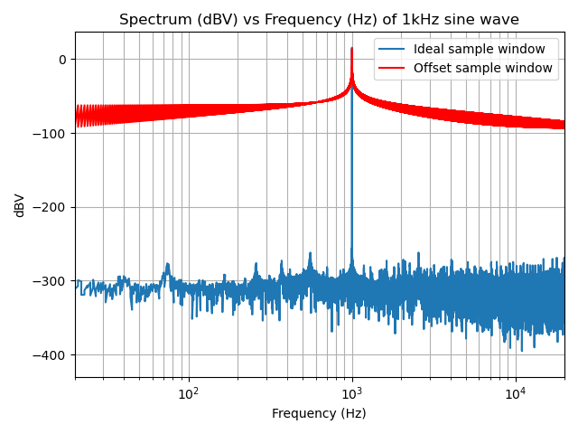
As you can see, this significantly impacts the DFT; the noise, which had been sitting down around -300dBV has been raised to around -80dBV! The main component of the spectrum is still at 1kHz, but it is nowhere near as nicely defined. This is due to the noise introduced by the rectangular window that causes the extended signal not to meet in a good way:
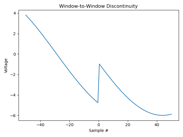
This plot shows the last 50 samples of the first sample window followed by the first 50 samples. Note that the “real” signal is a nice sine wave, this introduces a discontinuity; this is what causes the raised noise floor above.
Windowing
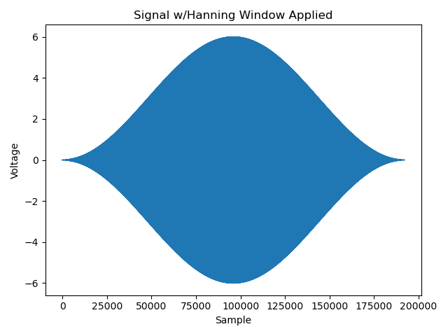
Windows are used to scale the input signal in a way that eliminates this discontinuity in a predictable way. One of the better known ones is the Hanning Window, that looks like this in the real domain:
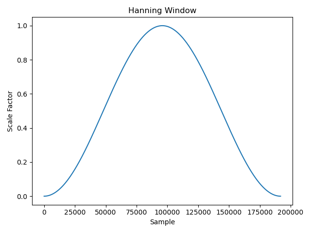
As you can see, this essentially forces the signal to zero at the beginning and end of the window when it is multiplied element-by-element with the input signal:
And while this appears to have altered the signal in a big way, let’s look at the spectrum to see that…
def reference_analysis():
    sample_rate_hz = 192 * 1000
    sample_time_s = 1.0/sample_rate_hz
    duration_s = 1
    n_samples = sample_rate_hz * duration_s
    amplitude_V = 6
    freq_hz = 1 * 1000
    t = np.linspace(0, duration_s - sample_time_s, num=n_samples)
    s = amplitude_V * np.sin(2 * np.pi * freq_hz * t)

    # Plot the ideal window signal
    s_fft = scipy.fftpack.rfft(s) * 2 / len(s)
    f_fft = scipy.fftpack.rfftfreq(len(s_fft), d=1 / sample_rate_hz)
    plt.plot(f_fft, 20*np.log10(np.abs(s_fft)), label='Ideal sample window')

    # Drop some samples at the beginning and end of the ideal samples
    first_sample = 101
    last_sample = len(s) - 67
    print('{} - {}'.format(first_sample, last_sample))
    windowed_samples = s[first_sample:last_sample]
    window_fft = scipy.fftpack.rfft(windowed_samples) * 2 / len(windowed_samples)
    f_window_fft = scipy.fftpack.rfftfreq(len(window_fft), d=1/sample_rate_hz)

    # Plot the FFT of the modified sample window
    plt.plot(f_window_fft, 20*np.log10(np.abs(window_fft)), color='r', label='Offset sample window')

    # Apply the hanning window and perform fourier transform
    window = np.hanning(len(windowed_samples))
    scaled_samples = window * windowed_samples
    hanning_fft = scipy.fftpack.rfft(scaled_samples) * 2 / len(scaled_samples)
    f_hanning = scipy.fftpack.rfftfreq(len(hanning_fft), d=1/sample_rate_hz)

    plt.plot(f_hanning, 20*np.log10(np.abs(hanning_fft * np.sqrt(8/3))), color='green', label='Offset w/Hanning')

    plt.xlabel('Frequency (Hz)')
    plt.ylabel('dBV')
    plt.xscale('log')
    plt.xlim([20, 20000])
    plt.grid(True, which='both')
    plt.title('Spectrum (dBV) vs Frequency (Hz) of 1kHz sine wave')

    plt.legend()
    plt.show()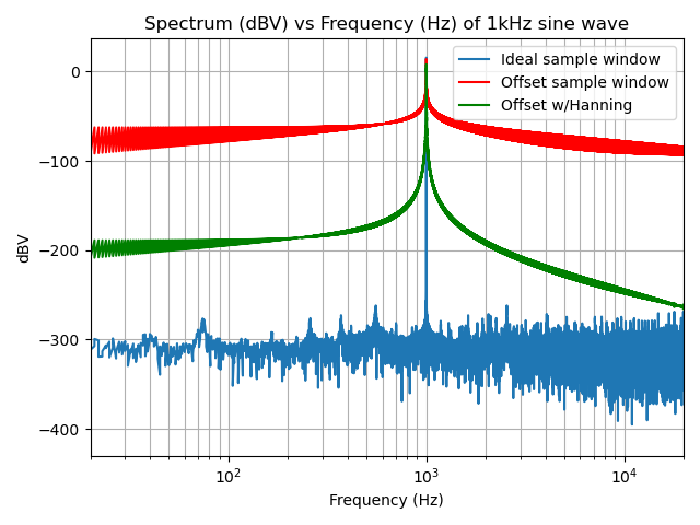
…the windowing actually didn’t really affect the shape of the spectrum all that much! It seems to have widened the “skirt” around the 1kHz signal relative to the noise floor (see Spectral Leakage), which isn’t great, but it pushed the noise floor down by over 100dBV. If you look closely, the peak value of the ideal spectrum above is 15.56dBV, 13.91dBV in the more realistic sample range and is now 8.03dBV with the Hanning window. The reason for this is Parseval’s Theorem, which roughly states that the energy contained in a signal is equal to the energy contained in the transform. In this example, as the peak falls, the energy is spread into the surrounding frequency bins, so that the overall energy doesn’t change, it is just arranged differently.
It is interesting to note is that the Hanning window appears to have its largest effect at higher frequencies. This makes sense, because the discontinuity outlined above appears in the frequency spectrum as a high frequency signal.
The Windowing throws away energy in the signal that we have to account for; the Hanning Window, for example, can be compensated
for by multiplying the amplitude of the DFT by sqrt(8/3). This isn’t perfect (due to the above-mentioned leakage) but it is pretty close.
Other Windows
There are many different windowing functions. Here are a few:
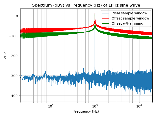
Hamming Window
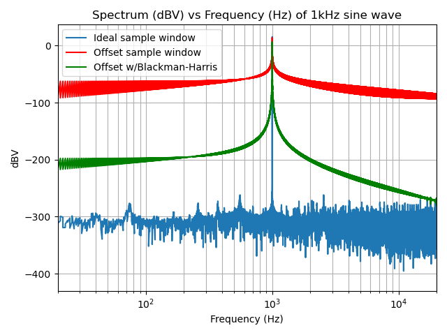
Blackman-Harris Window
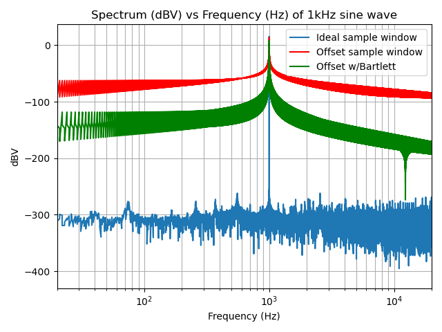
Bartlett Window
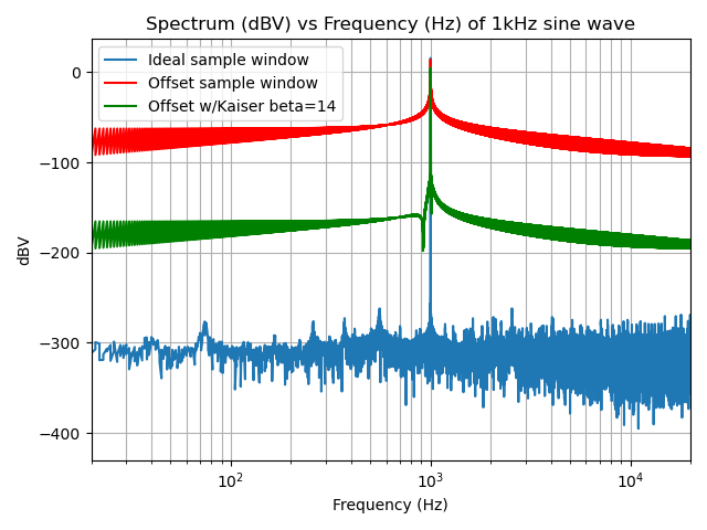
Kaiser Window (beta=14)
Summary
All of these windowing functions have their own quirks; I imagine that which one to choose depends a lot on its application and the type of signal that you’re applying it to. For my purposes, any filter that minimally affects the spectrum is best, while pushing the noise floor down below -150dBV. This is because my measuring equipment can’t get much below this (my Saleae is around -100dBV and I believe the AP analyzer I used recently to be around -140dBV). For this, the Hanning Window works well.