Quick Recap

I’ve decided to use an STM32 microcontroller to act as the USB to I2S interface. This requires (at least) three things:

1. USB handler to receive & buffer samples
2. Configure the PCM5242 to receive I2S samples
3. I2S output handler (to DAC)

This post will cover parts 2 and 3, to some degree. I intend to see how well I can output a “pure” sine wave from the STM32 to the DAC. I will be re-using the same DAC board as I made previously, which is one benefit of the modular approach I’ve taken for this project.

Configure the PCM5242

In this configuration, I will use I2C to configure the PCM5242 to accept 16-bit audio samples. I chose 16-bit because it fits nicely into memory; 24-bit audio would require an extra 0-byte due to the DMA controller requirements on the STM32F746ZG chip I am using.

Data Limitation

In order to reduce the processor burden on the STM32, I intend to utilize the memory-to-I2S interface DMA controller. This means I can essentially write data to memory, and allow the DMA controller to transfer that out the I2S interface correctly. The DMA controller can be configured to read from a memory address (the source) and write to a peripheral’s memory space (I2S, the destination).

We then must configure the data representation both at the source and the destination. If we were simply transferring 8-bit bytes, this is simple: read a byte from memory, write it to the peripheral. Where this gets hairier is in situations like 24-bit audio. The DMA controller does not support 24-bit reads, and the peripheral requires a 32-bit write to transfer 24 bits (i.e. it requires zero-padding to 32 bits regardless of the fact that it will only transfer 24 of them over the I2S bus).

What this means is that in memory we’d have to reserve bytes simply for padding; they do not get transferred over the wire, but they do need to be transferred via the memory bus. This is pretty inefficient, especially since I won’t be using external memory for this. In this case, it’s 1 useless byte for every 3 useful ones–not a great ratio.

If I end up really wanting to create 24-bit audio, I’ll circle back to this and probably sacrifice internal buffer time, but for now I’m going to stick to 16-bit data.

The 1kHz Sine Wave

One fairly standard test for audio DACs is how well they reproduce a full-scale sine wave at 1kHz. So let’s do this test!

The code for generating a sine wave is fairly straightforward:

static bool calculate_wave_samples(int16_t *samplePtr, int n_channels, int16_t amplitude,
        int n_samples, float *angle, float angle_delta)
{
    int i;
    int channel;

    assert(samplePtr != NULL);
    if (samplePtr == NULL)
        return false;

    assert(angle != NULL);
    if (angle == NULL)
        return false;

    for (i = 0; i < n_samples; i += n_channels, samplePtr += n_channels)
    {
        *samplePtr = amplitude * cosf(*angle);
        for (channel = 1; channel < n_channels; channel++)
        {
        	samplePtr[channel] = *samplePtr;
        }

        *angle += angle_delta;
        if (*angle > 2.0f * M_PI)
        	*angle -= 2.0f * M_PI;
    }

    return true;
}

There are a few things of note here. One is that this supports multiple channels (really just up to 2); the samples are packed either LLLLL or LRLRLR, so this could be a boolean, and in fact probably should be. However, I’m not going to worry about this right now. Next, this takes a pointer to the current angle variable; this is so that state is not preserved within the function, but someplace outside of it. This will be important later. Also, for some reason I chose to use cosf() rather than sinf(); this was just an arbitrary choice. However, note that these are the float-based functions rather than the double-based ones. This will be important later.

To test this, there is an easy way, and the “right” way. Let’s look at the easy test first:

The Easy Way

If we configure the DAC to run at a 48kHz sample rate, a 1kHz sine wave can be stored completely in memory in 96 samples (2 channels x 48kHz / 1kHz) = 96 samples. We can then configure the DMA controller to run in a circular loop, transferring the memory over and over again. This is a static example, and is fairly straightforward: precompute the sine wave, set up the DMA loop and start it, then sleep until the cows come home. I did this first, and things looked great on the scope!

The “Right” Way

In reality, we’re going to have to do some more fancy handling; the data will be coming in from USB and placed into the circular buffer while the DMA is transferring out data on the I2S interface. To approximate this, I wrote some code for the DMA interrupts that occur at the halfway point and at the end of the buffer transfer. In order to ensure that I am doing this correctly, I chose to use a 44.1kHz sample rate, which does not nicely divide into a small buffer size.

The logic to do this is then:

1. Pre-compute one full buffer length of audio samples (say, 100 samples worth).
2. Start the DMA transfer.
3. Interrupt fires when half of the samples have been transferred (in this example, when the 50th sample has been transferred). Compute the next 50 samples, storing them in the first half of the buffer.
4. Interrupt fires when the second half of the samples have been transferred (100th sample, in this example). Compute the next 50 samples, storing them in the second half of the buffer.

The functions to do this are as follows:

void HAL_I2S_TxHalfCpltCallback(I2S_HandleTypeDef *hi2s)
{
	// The first half has been transferred, overwrite that.
	if (!calculate_wave_samples(&m_InputWave[0], 2, INT16_MAX,
        MAX_WAVE_LEN / 2, &m_CurrentAngle_rad, m_AngleDelta_rad))
    {
	    while(1);
    }
}

void HAL_I2S_TxCpltCallback(I2S_HandleTypeDef *hi2s)
{
	// Calculate the second half of the wave
    if (!calculate_wave_samples(&m_InputWave[MAX_WAVE_LEN / 2], 2, INT16_MAX,
        MAX_WAVE_LEN / 2, &m_CurrentAngle_rad, m_AngleDelta_rad))
    {
        while(1);
    }
}

These function calls rely on some STM32 framework “magic”, which is a little annoying–the function names are weakly defined as empty functions, so unless the user implements them, nothing happens during the interrupt. However, we define them here to backfill the buffer as it is being DMA-ed out.

Pro Tip: Use the cosf() function, and not the cos() function. The cos() function is based on the double data type, which is incredibly slow (and unnecessarily high precision) on the STM32. When I first implemented this second method, I noticed on the oscilloscope that my sine wave had some significant discontinuities. I spent some time double-checking my math before I realized that I was simply falling behind. This was surprising to me, because I’d expect that it wouldn’t take more than 22.68usec to calculate a sample (1 samples @ 44.1kHz => 22.68usec), but apparently it does. To be fair, 64-bit double precision floating point is probably not something I should expect the STM32 microprocessors to do efficiently. In any case, switching to the float-based cosf() functions eliminated this problem.

Testing

So on the scope, everything looks great–we have a 4.2Vrms sine wave being output the right and left channels! How clean is that sine wave? Well, that’s a good question. One website I’ve been perusing uses an Audio Analyzer to characterize DACs, so in order to compare my work against existing devices, their methodology would be good. Unfortunately the ‘scope I have at home is pretty limited; it’s just two channels, both of which I use to plot the differential signal. I’d rather not add a breadboard or something to combine them into a single-ended wave, so how to measure this?

Saleae

In order to analyze the data a bit, I need a way to capture actual samples; my oscilloscope is fairly limited, so I don’t have a way to do the calculations on it (e.g. FFT of a differential signal). I decided to try using my Saleae’s analog inputs to capture some data. I set it up to sample two channels of analog input at +/- 5V at 1MHz for 5,000 samples. This seemed to work pretty nicely! However, my next issue is….what to do with this data?

A good start would be to simply examine the Fourier transform. I expect to see a spike at 1kHz (technically, at +/- 1kHz, due to the negative frequeny aspect, but since this is a real signal, the spectrum is conjugate symmetric, so I choose to consider only the positive frequencies).

def plot_simple_spectrum(time, samples):
    # Note: by inspection, the time sample data was *not* at fixed intervals, but had some jitter.
    # To make the plot below a bit more accurate, I simply grab the median of the time diffs.
    sample_time = np.median(np.diff(time))

    plt.subplot(2, 1, 1)
    plt.plot(time, samples)
    plt.xlabel('Time (s)')
    plt.ylabel('Sample (V)')
    plt.xlim([0, 0.050])
    plt.title('Samples vs. Time (First 50ms)')

    samples_fft = scipy.fftpack.rfft(samples) * 2 / len(samples)
    freq = scipy.fftpack.rfftfreq(len(samples_fft), d=sample_time)

    plt.subplot(2, 1, 2)
    plt.plot(freq, np.abs(samples_fft))
    plt.xlim([20, 20*1000])
    plt.xscale('log')
    plt.xlabel('Frequency (Hz)')
    plt.ylabel('Magnitude')
    plt.title('Audio Spectrum')
    plt.show()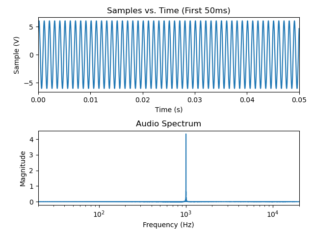

Ok, this matches my expectations; the biggest component of this signal is the 1kHz sine wave that I told the DAC to create. A standard way to look at an audio data spectrum is using a decibel scale. A decibel scale is a scaled ratio, so we need to use something as the reference. In this case, a standard one is 1V, which we can scale as dBV. The math for this is simple, since we simply divide the signal (in Volts) by the reference voltage (1V) and then convert to decibels: 20*log10(abs(fft(data))). Doing this yields the following plot:

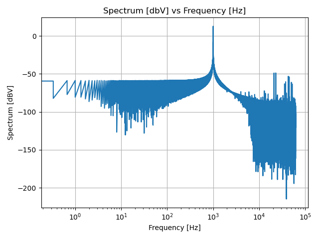
This plot reveals that there’s a lot of noise at about -60dBV across the spectrum. Where is this coming from? One area is from the sampling window we’re using. Since a DFT is done assuming that the data sample repeats ad infinitum, some artifacts are introduced if the sampling window isn’t exactly right (e.g. the last sample doesn’t perfectly line up with the first sample). One way to dimish this effect is via windowing.

Essentially, windowing intentionally dimishishes the input signal in a predictable way to make it truly periodic. This introduces its own artifacts, but these artifacts are known and can be accounted for (e.g. this dimishes the energy in the signal, but in a known way, so the resultant DFT can be corrected for the lost energy).

A widely-used window is the Hanning Window. The result of applying this window is the following plot:

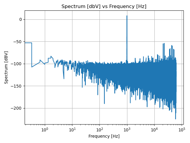
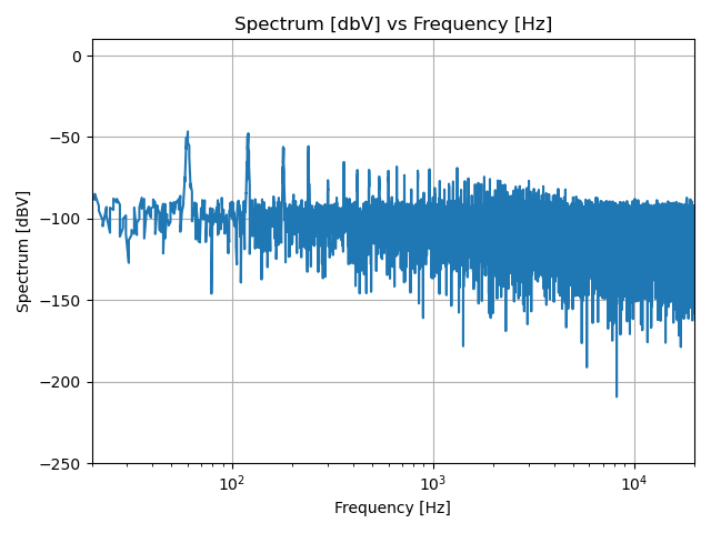
As is evident, this pushes the “noise floor” down from about -60dBV to about -90dBV – not too shabby! Let’s adjust the plot to just the frequencies we care about; since this is audio, I’ve chosen 20Hz - 20kHz. There are audiophiles out there that don’t like to do this, as they feel it isn’t as pure a picture of performance as the complete spectrum, but I’m choosing to focus on this area for now.

Now, as I mentioned before, this Hanning window has the effect of diminishing the signal; we need to account for the lost energy in some way. The Hanning window is well known, and the factor to apply in the frequency spectrum is sqrt(8/3). This doesn’t change the graph much, so I haven’t included it here.

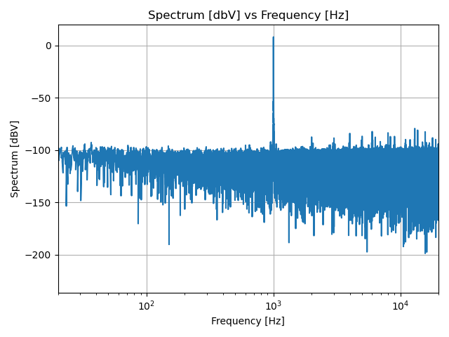
Inspecting this graph, it appears that the 1kHz signal is sitting nicely at 4 dBV, and the noise floor is around -95dBV, so if you want a measurement of signal quality, you could say SNR is around 4 dbV - (-95dBV) = 99dbV. Not too shabby.

Noise Floor

So, now the question is: is the Noise Floor of my DAC at -95dBV, or is the Noise Floor of my Saleae’s Analog Inputs at -95dBV? To test this, I disconnected the probes of my Saleae and measured them. Plotting the data in the same way as above, we see the following:

Based on this graph, it appears that my DAC’s precision is higher than the Saleae can reliably measure. This makes sense to me, since the Saleae is a protocol analyzer, and really is designed for digital signals. I don’t think I can say a whole lot about the noise floor of my DAC since it would appear to be lower than the Saleae’s.

THD+N

Lastly, I’m interested in the Total Harmonic Distortion Plus Noise, also known as THD+N. This is a calculation of the amount of energy due to the fundamental frequency relative to the total energy contained in the spectrum. There are a few ways to calculate this, but I’m choosing to do it in the frequency domain because it makes the math easier.

The THDN is fairly simple to calculate: it is the ratio of all of the RMS of all of the signal except for the fundamental divided by the RMS of all of the signal.

THDN = V_rms_masked / V_rms

My python code for calculating the THDN is as follows:

def calculate_thdn(freq, spectrum_fft, fundamental=1000, fundamental_skirt=50):
    # We only wish to calculate THDN from 20-20kHz.
    freq_mask = np.ma.masked_outside(freq, 20, 20000)
    freq_valid = freq_mask.compressed()
    spectrum_fft_valid = spectrum_fft[~freq_mask.mask]

    whole_rms = np.sqrt(2 * np.sum(np.abs(spectrum_fft_valid) ** 2))
    print('RMS: {}'.format(whole_rms))

    # Mask out the fundamental frequency +/- a skirt
    freq_noise_and_harmonics_mask = np.ma.masked_inside(freq_valid, fundamental - fundamental_skirt,
                                                        fundamental + fundamental_skirt)
    fft_nh = spectrum_fft_valid[~freq_noise_and_harmonics_mask.mask]
    masked_rms = np.sqrt(2 * np.sum(np.abs(fft_nh) ** 2))
    print('Masked RMS: {}'.format(masked_rms))

    thdn_unscaled = masked_rms / whole_rms
    print('THDN (Unscaled): {}'.format(thdn_unscaled))
    print('THDN (%): {:02f}'.format(thdn_unscaled * 100))
    print('THDN (dB): {}'.format(20 * np.log10(thdn_unscaled)))

Using the same data as above (sourced via the Saleae’s Analog Inputs), this code produced the following output:

RMS: 8.516772283265139
Masked RMS: 0.002980010514717971
THDN (Unscaled): 0.0003498990480904935
THDN (%): 0.034990
THDN (dB): -69.12114478049953

According to the folks at Audio Precision, the way to present this is as follows: THD+N less than 0.035%, 6Vrms, 20 Hz - 20 kHz, unity gain, 20 kHz BW. Note that this is probably somewhat worse than the DAC actually is, because as I showed previously, the noise floor of the Saleae is higher than the noise floor of the DAC.

Let’s compare these results against a calibrated Audio Analyzer!

Audio Analyzer

Well, I do work at an audio company. I asked a coworker to help characterize my DAC and he introduced me to the Audio Precision APx58x analyzer. I checked eBay to see if I could maybe pick up a used one for something reasonable (say under $1,000). Yeah, that won’t happen–they run somewhere well north of $20k. In any case, I was able to use the one at work to take a look at the DAC outputting the sine wave.

Sine Wave Output

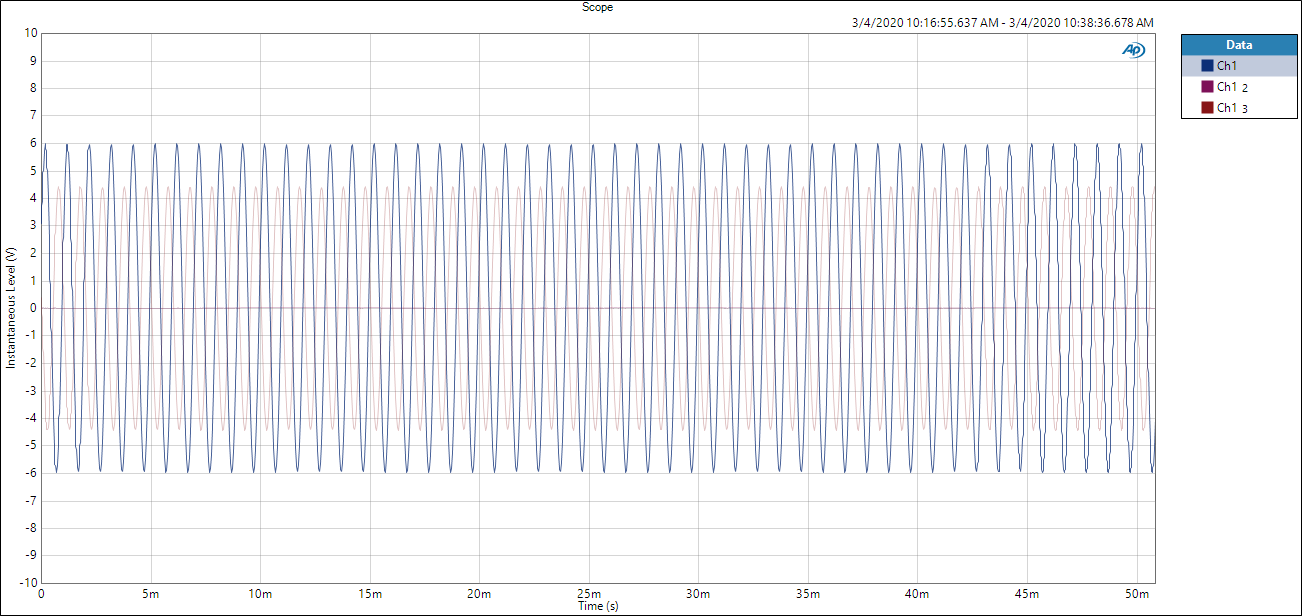
The first results were… disappointing. This is represented by the light pink signal above. There was clearly something wrong here–the signal was a full-scale sine wave @ 4.2Vrms–this should be sqrt(2) * 4.2 = 6V peak voltage. But I’m only seeing ~4.3V for some reason. The first thing to come to mind was that perhaps my power supply was doing something bad. The STM32/DAC was plugged into a Dell laptop’s USB port I know that USB ports can be pretty crappy, especially on some Dell laptops (my Mac has never given me trouble on this–I don’t know about other PC manufacturers). I went to grab a battery, to test the STM32/DAC in isolation. This could be done because the sine wave is being generated on the STM32 itself, so there was no connection needed to a PC, I just needed the 5V power from somewhere.

With the battery (basically a phone charger), we re-characterized the system. Much better. Much better. As seen on the same graph above, the sine wave was now a full +/- 6V, with no visible clipping.

Spectrum Analysis

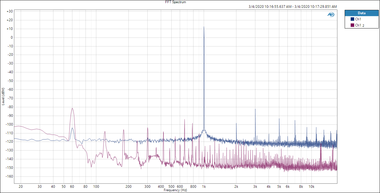
This chart shows two FFT plots, one of the DAC output (blue) and one of the ambient noise (the DAC was powered off) (purple). My relatively naive reading of this is that the noise floor of my DAC is roughly -120dBV, and the 1kHz sine wave is at roughly 14dBV–not too shabby! The harmonics of the 1kHz signal are clearly visible, as is some noise at 60Hz (I’m in the US, so that’s likely noise coupled from the fluorescent lights or electrical wiring in the walls). Interestingly, the 60Hz noise was diminished nicely on my measurement, so clearly the grounding isn’t totally crap.

Total Harmonic Distortion + Noise

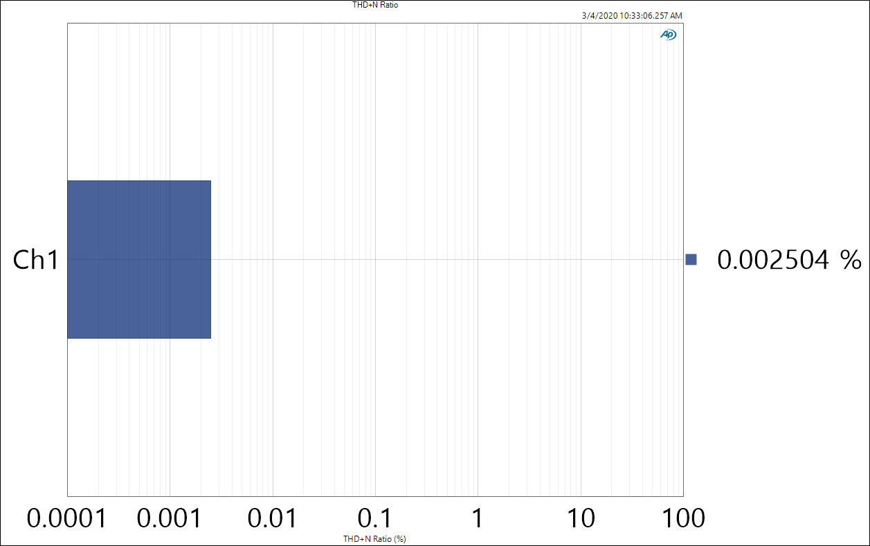
Finally, we have the THD+N Ratio. This is a ratio of the total energy outside of the desired signal (1kHz) against the energy in the desired signal, so lower is better. In this case it’s a nice 0.002504%, which seems low. Is it? I don’t really know. Based on the Audio Science Review website reviews above, it seems pretty good – low enough not to introduce audible artifacts. Note that this measurement was only taken in the audible band (up to 20kHz). It may be more correct to expand that window to higher frequencies, but to me it didn’t seem obvious that this was the case. Also, it made my number look worse, so….

Takeaways

I need to find a way to ensure that I can handle a crappy USB port up-stream. I’m not sure if this means better grounding, more power-cleanup stages or what, but clearly this is going to be an issue. None of the things I’m doing should require more the 2.5W (500mA x 5V) that USB 2.0 allows, so hopefully it’s a matter of adding better filtering to the ground / power rails.

However, I am very encouraged that the performance is seemingly pretty good in isolation! Granted, I haven’t really proved anything except that yep, the data sheet wasn’t lying, but that’s still a nice feeling to see a clean sine wave.

Comparing my own Saleae measurements against the AP Analyzer, it seems that my DAC’s performance is simply better than the Saleae can measure. This is fair, considering that the Saleae really wasn’t designed for this sort of analysis.

Now that I have a 1kHz sine wave working, I just need to fill in all of the other frequencies! But seriously, the next step is to hook up the USB audio transfers to the buffer that the DMA engine is reading from. I expect that at a first pass this will be fairly straightforward, but that the devil will be in the details (what to do about clock drift? what do we do if/when we under- or overrun?)